As I've been learning more about different types of models, I thought: why not see how I can use logistic regression to classify my dear cat Goldie? I have hundreds of photos of Goldie on my phone, surely enough to train a model and do some binary classification with. Without further ado, let's get into it.
Data set-up
I started with two folders: ~400 images of Goldie and ~400 random images pulled from Unsplash via their API. Each image gets cropped to a square (so nothing looks stretched), resized to 128×128, flattened, and standardised by dividing by 255. Goldie gets label 1, everything else 0.
def load_images(folder, label, img_size=(128, 128)):
    images, labels = [], []
    for filename in os.listdir(folder):
        if filename.lower().endswith((".jpg", ".jpeg", ".png")):
            img = Image.open(os.path.join(folder, filename)).convert("RGB")
            # center-crop to a square, then resize
            w, h = img.size
            if w != h:
                m = min(w, h)
                left, top = (w - m) // 2, (h - m) // 2
                img = img.crop((left, top, left + m, top + m))
            img = img.resize(img_size)
            images.append(np.array(img))
            labels.append(label)
    return images, labels
A quick look
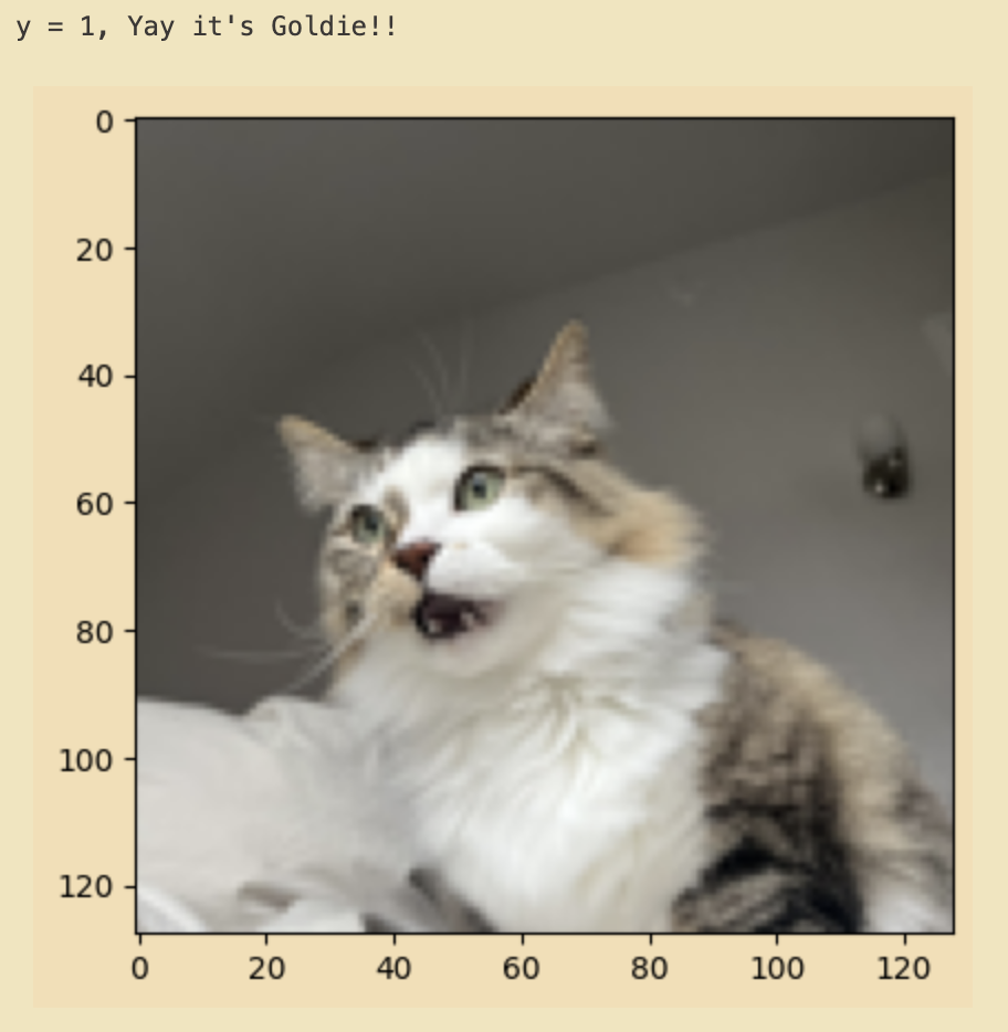
Before training, I like to eyeball a few examples to make sure the labels line up with the pictures.
Forward & backward propagation
Now for the cost function and gradients. I used L1 regularization (Lasso) on the intuition that pixels near the edges of a photo shouldn't matter as much as the centre, since Goldie is usually near the middle of the frame. Without regularization, both train and test accuracy were ~15% worse.
The cost function with the L1 penalty:
J(w,b) = (1/m) Σ [ −y·log(a) − (1−y)·log(1−a) ] + (λ/m) Σ |wj|
σ(z) = 1 / (1 + e−z), z = wᵀx + b
def propagate(w, b, X, Y, lambda_reg):
    m = X.shape[1]
    A = sigmoid(np.dot(w.T, X) + b)
    A = np.clip(A, 1e-10, 1 - 1e-10)          # avoid log(0)

    cost  = (-1/m) * np.sum(Y*np.log(A) + (1-Y)*np.log(1-A))
    cost += (lambda_reg/m) * np.sum(np.abs(w)) # L1 penalty

    dw = (1/m) * np.dot(X, (A - Y).T) + (lambda_reg/m) * np.sign(w)
    db = (1/m) * np.sum(A - Y)
    return {"dw": np.clip(dw, -1, 1), "db": np.clip(db, -1, 1)}, np.squeeze(cost)
Gradient descent then just nudges w and b down the cost surface for a fixed number of iterations, recording the cost as it goes.
Results
I ran 5,000 iterations at a learning rate of 0.001. A higher rate (0.1 or 0.01) made the cost jump all over the place; dropping to 0.001 finally gave a smooth descent. Here's the cost over training: