Logistic Regression: Goldie Versus The World
As I’ve been learning more about different types of models, I thought, why not try to see how I can use logistic regression to classify my dear cat Goldie. I have hundreds of photos of Goldie on my phone, surely enough to train a model and do some binary classification with. Without further ado, let’s get into it!
# Load packages
import numpy as np
from proj_fcns import sigmoid, initialize_parameters, plot_costs
import os
import matplotlib.pyplot as plt
from PIL import Image
Data set up
Let’s begin by creating our dataset. I already have two folders that contain ~400 images of goldie and 400 random images collected from Upsplash using their API (see github for image collection process).
Since I have all the images I want to use, I want to bring them in as arrays where each RGB value is recorded for each pixel for every images. I then want to assign the label 1 to all my Goldie images and 0 to all the random non-Goldie images.
I’m also going to crop every images so the aspect ratio is consistent (don’t want the images to look stretched or squished) and divide each images into 128 by 128 pixels.
def load_images(folder, label, img_size=(128, 128)):
    """
    Loads images from a folder and assigns them a label.

    Parameters:
        folder (str): Directory containing images.
        label (0 or 1): Label assigned to each image.
        img_size (tuple): dimentions to resize images (width, height). Default is (128, 128).

    Returns:
        tuple: Lists of preprocessed images and their labels.
    """
    images = []
    labels = []
    for filename in os.listdir(folder):
        if filename.endswith(".jpg") or filename.endswith(".jpeg") or filename.endswith(".png"):
            img_path = os.path.join(folder, filename)
            img = Image.open(img_path).convert('RGB')  # Convert to RGB

            # Crop the image to a square
            width, height = img.size
            if width != height:
                if width > height:
                    left = (width - height) // 2
                    right = left + height
                    top = 0
                    bottom = height
                else:
                    top = (height - width) // 2
                    bottom = top + width
                    left = 0
                    right = width
                img = img.crop((left, top, right, bottom))

            # Resize the image to the desired size
            img = img.resize(img_size)

            img_array = np.array(img)
            images.append(img_array)
            labels.append(label)
    return images, labels

base_path = os.getcwd()

# Construct the relative path to the images folder
cat_folder = os.path.join(base_path, "images", "goldie_pics")
not_cat_folder = os.path.join(base_path, "images", "random_pics")

# Load images
cat_images, cat_labels = load_images(cat_folder, 1)
not_cat_images, not_cat_labels = load_images(not_cat_folder, 0)

# Combine the datasets
all_images = np.array(cat_images + not_cat_images)
all_labels = np.array(cat_labels + not_cat_labels)

# Shuffle the dataset
shuffle_indices = np.random.permutation(len(all_labels))
all_images = all_images[shuffle_indices]
all_labels = all_labels[shuffle_indices]

# Split into training and testing sets (80% train, 20% test)
split_index = int(0.8 * len(all_labels))
train_images = all_images[:split_index]
train_labels = all_labels[:split_index]
test_images = all_images[split_index:]
test_labels = all_labels[split_index:]

# Reshape
train_images_flatten = train_images.reshape(train_images.shape[0], -1).T
test_images_flatten = test_images.reshape(test_images.shape[0], -1).T

# Standardize
train_set = train_images_flatten / 255.
test_set = test_images_flatten / 255.
Test images
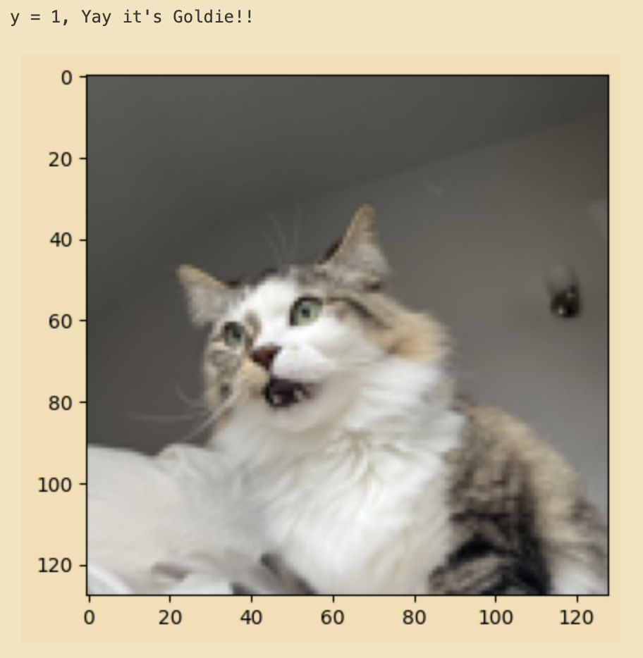
To make sure the images look good loaded in, let’s just take a quick look at a few examples to see what we’re working with.
index = 2 # Change index to see what different pics are in the dataset!
plt.imshow(train_images[index])

if train_labels[index] == 1:
    result = "Yay it's Goldie!!"
else:
    result = "Boo, not a Goldie pic"

print ("y = " + str(train_labels[index]) + ", " + result)

Reshape and standardize
Now let’s do some organization. We want a 2D array so let’s reshape and standardize our data. To standardize, I’m dividing by 255 since the RGB values range from 0 to 255.
# Reshape
train_images_flatten = train_images.reshape(train_images.shape[0], -1).T
test_images_flatten = test_images.reshape(test_images.shape[0], -1).T

# Standardize
train_set = train_images_flatten / 255.
test_set = test_images_flatten / 255.
Propogation
Now I want to compute the cost function and gradients using forward and backward propogation.
I’m going to use regularization for this to prevent overfitting. Without regularization, both the training and test accuracy of the model was ~15% less accurate! A model that can only detect a goldie image two thirds of the time is not that much better than random chance!
I’m choosing to use L1 regularization (Lasso Regression) with the idea that the pixels on the outside of the image should not have as much impact on image classification as the images near the centre of the image. I believe most images of Goldie shoud be (at least somewhat) centred.
This means the cost function is going to look a little different - there’s an added term at the end which adds the sum of the absolute value of the weights to the cost function. Here’s what the cost function now looks like:
$$ J(w, b) = \frac{1}{m} \sum_{i=1}^{m} \left[ -y^{(i)} \log(a^{(i)}) - (1 - y^{(i)}) \log(1 - a^{(i)}) \right] + \frac{\lambda}{m} \sum_{j=1}^{n} |w_j| $$
Also, note the sigmoid function: $$\sigma (z) = \frac{1}{1 + e^{-z}} \quad \text{where} \quad Z = w^T x + b$$ is used to map the values between 0 and 1 so the results can be interpreted as a probability.
def propagate(w, b, X, Y, lambda_reg):
    """
    Implements forward and backward propagation for the model.

    Parameters:
        w (ndarray): Weights, shape (dim, 1).
        b (float): Bias.
        X (ndarray): Input data, shape (dim, number of examples).
        Y (ndarray): True labels, shape (1, number of examples).
        lambda_reg (float): Regularization parameter.

    Returns:
        tuple: Gradients (dict with "dw" and "db") and cost.
    """
    m = X.shape[1]

    # Forward propagation
    A = sigmoid(np.dot(w.T, X) + b)

    # Add epsilon to avoid log(0) issues
    epsilon = 1e-10
    A = np.clip(A, epsilon, 1 - epsilon)

    # Cost function
    cost = (-1/m) * np.sum(Y * np.log(A) + (1 - Y) * np.log(1 - A))
    cost += (lambda_reg / m) * np.sum(np.abs(w))  # L1 Regularization term

    # Backward propagation
    dw = (1/m) * np.dot(X, (A - Y).T) + (lambda_reg / m) * np.sign(w)  # L1 Regularization term
    db = (1/m) * np.sum(A - Y)

    # Clip gradients to avoid massive gradients
    dw = np.clip(dw, -1, 1)
    db = np.clip(db, -1, 1)

    cost = np.squeeze(cost)
    grads = {"dw": dw,
             "db": db}

    return grads, cost
Optimization
The aim is to minimize the cost function
To do this, the propogation function defined above is used to get the current gradients for the weights (dw) and bias (db). These values are used in gradient descent to calculate the cost. With each iteration, weights and bias will get updated to minimize the cost.
def optimize(w, b, X, Y, num_iterations, learning_rate, lambda_reg, print_cost=False):
    """
    Optimizes parameters using gradient descent.

    Parameters:
        w (ndarray): Weights, shape (dim, 1).
        b (float): Bias.
        X (ndarray): Input data, shape (dim, number of examples).
        Y (ndarray): True labels, shape (1, number of examples).
        num_iterations (int): Number of iterations for optimization.
        learning_rate (float): Learning rate for gradient descent.
        lambda_reg (float): Regularization parameter.
        print_cost (bool): If True, prints cost every 100 iterations. Default is False.

    Returns:
        tuple: Optimized parameters (dict with "w" and "b"), gradients (dict with "dw" and "db"), and list of costs.
    """
    costs = []

    for i in range(num_iterations):
        grads, cost = propagate(w, b, X, Y, lambda_reg)

        dw = grads["dw"]
        db = grads["db"]

        w = w - learning_rate * dw
        b = b - learning_rate * db

        if i % 100 == 0 or i == num_iterations - 1:
            costs.append(cost)
        if print_cost and (i % 100 == 0 or i == num_iterations - 1):
            print(f"Cost after iteration {i}: {cost}")

    params = {"w": w, "b": b}
    grads = {"dw": dw, "db": db}

    return params, grads, costs
Make Predictions
The follow function will be used to make the predictions - if we get a value over 0.5 then an image of Goldie is predicted! Otherwise it’s predicted to be a random, non-goldie image.
def predict(w, b, X):
    """
    Predicts labels for input data using learned parameters.

    Parameters:
        w (ndarray): Weights, shape (dim, 1).
        b (float): Bias.
        X (ndarray): Input data, shape (dim, number of examples).

    Returns:
        ndarray: Predicted labels, shape (1, number of examples).
    """
    m = X.shape[1]
    Y_prediction = np.zeros((1, m))
    w = w.reshape(X.shape[0], 1)

    A = sigmoid(np.dot(w.T, X) + b)

    for i in range(A.shape[1]):
        Y_prediction[0, i] = 1 if A[0, i] > 0.5 else 0

    return Y_prediction
Train the model
def model(X_train, Y_train, X_test, Y_test, num_iterations=2000, learning_rate=0.5, lambda_reg=0.1, print_cost=False):
    """
    Builds and trains a logistic regression model, then evaluates it on the test set.

    Parameters:
        X_train (ndarray): Training data, shape (dim, number of training examples).
        Y_train (ndarray): Training labels, shape (1, number of training examples).
        X_test (ndarray): Test data, shape (dim, number of test examples).
        Y_test (ndarray): Test labels, shape (1, number of test examples).
        num_iterations (int): Number of iterations for optimization. Default is 2000.
        learning_rate (float): Learning rate for gradient descent. Default is 0.5.
        lambda_reg (float): Regularization parameter. Default is 0.1.
        print_cost (bool): If True, prints cost every 100 iterations. Default is False.

    Returns:
        dict: Dictionary containing model information including costs, predictions, parameters, learning rate, number of iterations, and regularization parameter.
    """

    w, b = initialize_parameters(X_train.shape[0])

    parameters, _, costs = optimize(w, b, X_train, Y_train, num_iterations, learning_rate, lambda_reg, print_cost) # gradient dosn't need to be assigned

    w = parameters["w"]
    b = parameters["b"]

    Y_prediction_train = predict(w, b, X_train)
    Y_prediction_test = predict(w, b, X_test)

    print("train accuracy: {} %".format(100 - np.mean(np.abs(Y_prediction_train - Y_train)) * 100))
    print("test accuracy: {} %".format(100 - np.mean(np.abs(Y_prediction_test - Y_test)) * 100))

    d = {"costs": costs,
         "Y_prediction_train": Y_prediction_train,
         "Y_prediction_test": Y_prediction_test,
         "w": w,
         "b": b,
         "learning_rate": learning_rate,
         "num_iterations": num_iterations,
         "lambda_reg": lambda_reg}

    return d
Training
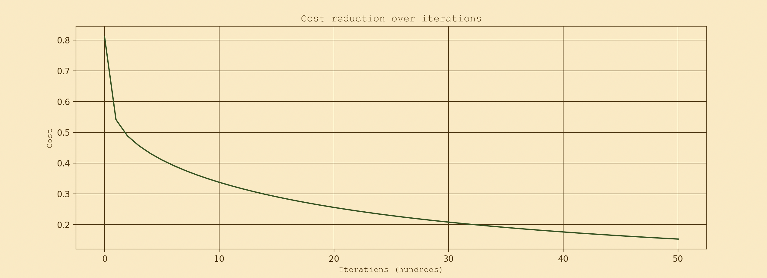
I’m going to do 5000 iterations to see how the model runs and plot the costs over iterations
# Reshape labels
train_labels = train_labels.reshape(1, -1)
test_labels = test_labels.reshape(1, -1)

# Train the model
d = model(train_set, train_labels, test_set, test_labels, num_iterations=5000, learning_rate=0.001, lambda_reg=0.01, print_cost=True)

# Plot the costs
plot_costs(d["costs"])
Results
Cost after iteration 4999: 0.15570564061677383
train accuracy: 97.70642201834862 %
test accuracy: 79.8780487804878 %
Nearly 80%, not too bad! Before adding in the regularization term, the test accuracy was a grim 65% so this is looking much nicer. I found of all the things I added to the simplist version of a logistric regression model, the regulairization term improved the accuracy the most. I also found the cost was jumping all over the place with each iteration when I had the learning rate at 0.1 and 0.01. When I decreased it even further to 0.001, the costs finally started to look at lot smoother so I kept it there. Take a look at the plot of the costs!
